The Effects of the Bishop Hill Illinois Wind Farm on Near-Surface Wind Patterns


Project poster presented at various conferences. This project took first place at the 18th Annual Severe Storms and Doppler Radar Conference hosted by the National Weather Association, earning the Tim Samaras Award for Best Student Poster. The award also took third place at the 14th Annual Student Conference in conjunction with the 95th Annual American Meteorological Society meeting.
Abstract
Wind energy is becoming a larger part of American energy production as wind farms are popping up all over the Midwest, particularly in Illinois, with large groupings of towering wind turbines. While these wind farms are forms of clean energy, they do create unintended effects to the winds around the turbines, and these effects can impact the efficiency of other wind turbines. The purpose of this research is to look at, in high resolution, the wind field around the Bishop Hill, Illinois wind farm and see its effects on the surrounding wind structure. Using the high-resolution radar on the Doppler on Wheels, the horizontal and vertical wind profile around the wind farm is analyzed using PPI and RHI scanning methods. The primary area of research is down wind of the turbines looking at the wake turbulence generated. Using the radar, downstream wind patterns were influenced by the wind turbines as well as the wind structure over the wind farm. Pockets of lesser wind velocities are seen directly correlated to the locations of wind turbines. Turbulence was also generated behind larger groupings of wind turbines. The data collected can be used to look at future placement of wind turbines to help increase their efficiency.
Introduction
The DOW project that we sent out to work on involved the DOW, wind, and a wind farm. We wanted to know how wind changes both in the vertical and in the horizontal as it moved through a wind farm. Shae was looking for any possible insect movement through the wind farm. Nick was looking for turbulence created by the wind farm down wind of the area. Anthony is looking at how the downstream winds compare to the upstream winds.
When we first thought of the idea for the wind farm, we wanted to scan six different location with both PPI and RHI scanning methods. We soon found out that was impossible in the allowed time frame for our project. We decided upon one deployment location that would best benefit all three research projects.
We had two deployment spot and they where located N 41.122869, W 90.250714 at an elevation 249m, and the second and final spot was N 41.129677, W 90.188393 at an elevation of 240m. We arrived at our first deployment site at 2:56 pm and tried to scan, but we had a few problems with the original site as we had power lines being picked up by the radar beam, as well as the fact the wind farm was in the “zero band” of our radar.
The zero band is the area in the velocity data of the radar where the wind is perpendicular to the radar vector. When the wind is perpendicular to the radar vector, there is no velocity data. The bad velocity data in the zero band was right over the wind farm therefore we could not get good velocity data.
We then proceeded to move to our second and final spot. We arrived to the second deployment site at 4:19 pm and this site was almost perfect for our project as it was between open fields and power lines were not between us and the wind farm. Conditions for our project where favorable for measuring winds through the wind farm with strong southeasterly winds at 5-10 miles per hour with gusts approaching 20 miles per hour as seen in figure 8.1.
Site Selection/Study Area Description
When we first arrived at our site to scan, it was approximately 2:30 p.m. We were level and ready to scan at 2:56 p.m. We left shortly thereafter at approximately 3:30 p.m. in search of a new location to scan due to the wind farm being in the “zero band” while scanning. We arrived at our second spot at approximately 3:45 p.m. After a short drive we were level and ready to scan at 4:19 p.m. After running both an RHI and PPI radar scans, we stopped the radar scanning at 4:53 p.m. and we were on our way back to Macomb by 5:30 p.m.
Deployment Site 1:

Fig. 1: The DOW location at the first deployment site in relation to the wind farm.
Our first deployment site was on N 2800 Rd. just west of E 1000 Rd. in Knox County. Our coordinates of our first deployment site was N 41.122869 W 90.250714 at an elevation of 249m.
An overview of the site given in Fig. 1 show that this was an ideal location. It was sitting higher up on a slight hill with a great view of the wind farm. As we take a closer look, there was a slight problem with the site, and that was power lines. In rural Illinois is is very difficult to avoid power poles on every road, and unfortunately on this road they were in between our radar and the wind farm.
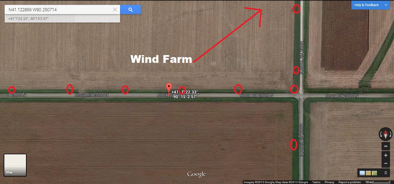
Fig 2: The deployment with the likely ground clutter sources highlighted. Each circle is a utility pole.
Fig. 2 highlights the utility poles that would be affecting our radar data acting as ground clutter.

Fig 3: Photo from the ground indicating the utility pole with the wind farm in the background. This pole would create a ground clutter return on the radar image.
Actually looking at photos from the ground, visually the elevation we have looking slightly down on the wind farm is visible in Fig. 3, and one of many power poles that would cause ground clutter on the radar images is seen. At this location, the power poles would be the dominant ground clutter objects.
Deployment Site 2:

Fig 4: An overview of the second deployment site in relation to the wind farm.
Our second deployment site was facing east on N 2850 Rd. between E 1240 and E 1350 Rd in Know County. The coordinates of the location were N 41.129677 and W 90.188393 at an elevation of 240m.
An overview of the site shown in Fig. 4 shows that this was a better location than the first location. Like the first location, it was on a hill, however at this site the power lines are on the other side and not blocking the view of wind farm.

Fig 5: Close up view of the second deployment site indicating the sources of ground clutter. Trees and utility poles are are highlighted.
A closer look at our second location in Fig. 5 shows the ground clutter that will show up on the radar scans. The primary ground clutter sources will be the power poles east of the DOW on the road, as well as the grouping of trees west of the DOW on the south side of the street. For us, this will have little impact on the radar data as what we are interested in is unobstructed to the north of the road.

Fig 6: Photo from the ground showing the causes of ground clutter on the radar returns.
A look actually on the ground in Fig. 6 shows the trees behind the DOW that would obstruct that radar data and cause ground clutter.
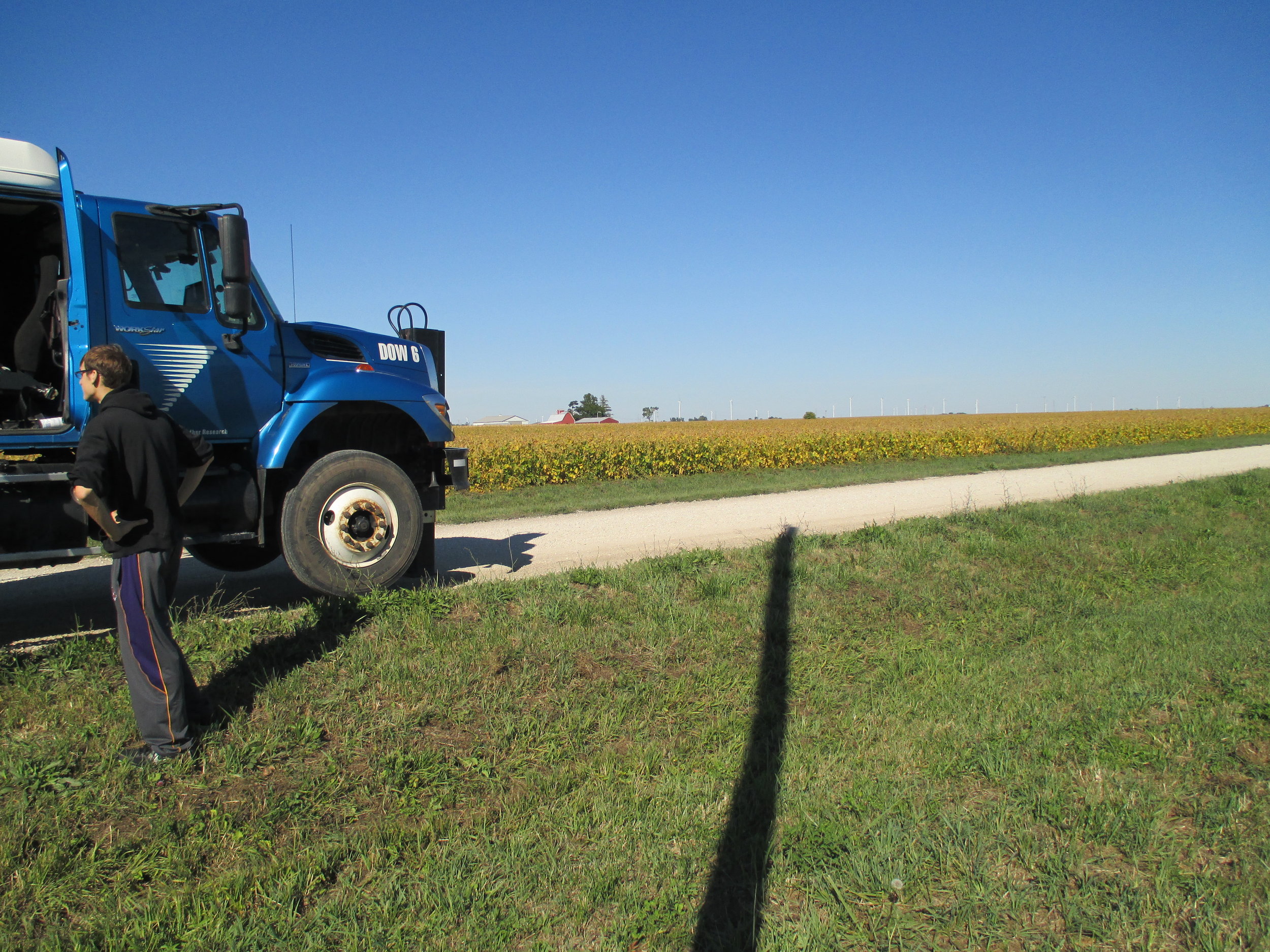
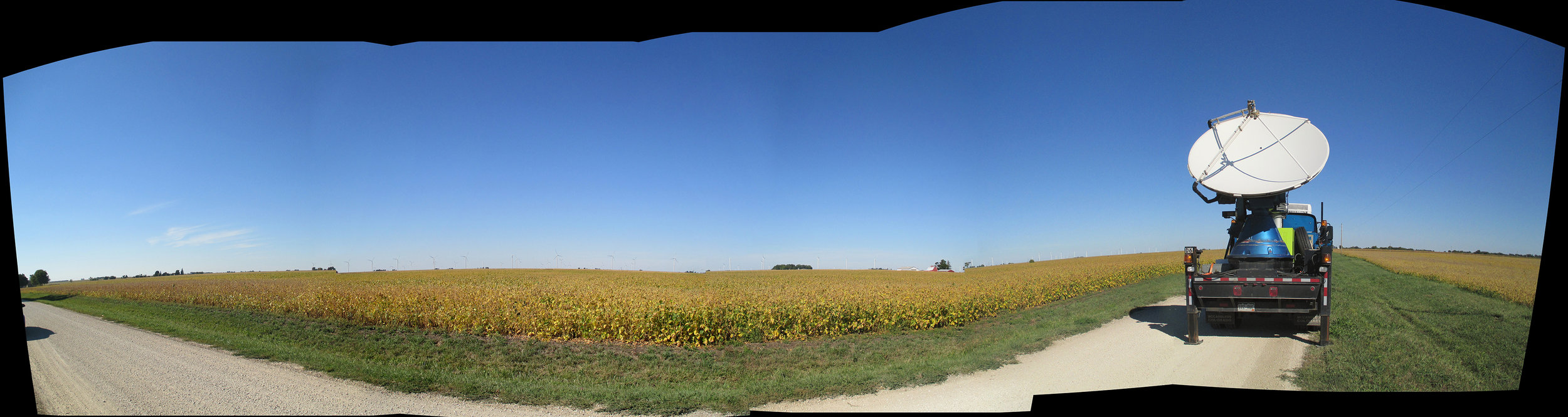
Fig 7: A full view looking towards the wind farm showing the unobstructed view of the radar.
Fig. 7 shows the full unobstructed view the DOW had of the wind farm off to the north. Ground clutter here could be the wind turbines themselves, however the radar angle should be high enough to be above the turbines.
Deployment Site Qualities
The good qualities of our second and main deployment site would be its location on a hill with a great perspective on the wind farm. The DOW has a full unobstructed view of the wind farm with no ground clutter that may obstruct the radar data.
While there were many great aspects of the deployment site, there were a few issues. We were fairly close to a home with trees surrounding the house, so any data to the SW will likely be obstructing the radar data. We also had power poles on the south side of the road that would obstruct the wind approaching us.
Atmospheric Conditions

Fig 8.1: The surface weather conditions from the closest reporting station to our site, Galesburg, IL, highlights the surface weather conditions.
Using the Wunderground Weather Archive for Galesburg, IL, which is the closest reporting station to our deployment sites, atmospheric conditions were fairly constant during the experiment. In figure 8.1 the weather data is shown, with the red box highlighting the time when we were scanning.
Winds were from the south when we first arrived before switching more southeast while we were scanning. Wind speed was fairly constant between five and ten miles per hour, peaking between 4:00 and 4:30 as shown in figure 8.1.
It was mostly sunny for the duration of the event with a few alto-cirrus clouds passing through.

Figure 8.2: A skew-t from the closest weather balloon launch site, Lincoln, IL, showing the stable atmospheric conditions.
Looking at the Lincoln, IL sounding in figure 8.2 at 7pm on the 24th, it shows a very stable environment for the area while we were scanning. The Skew-T can be seen below. CAPE is a staggering 2 j/kg.
The environment was quite dry while we were scanning, less than 50% humidity show in figure 8.1.
DOW in Action
Once we arrived to the scanning location, we are looking for a location to set up and scan. Once we parked on the side of the road, we had to go through the process of leveling the truck. The DOW has five hydraulic lift legs that allow the DOW to level itself at almost any location. They can each be manually controlled. The truck was originally leveled at location 1 (Fig 9.1), but was not fully level at location 2 (Fig 9.2).
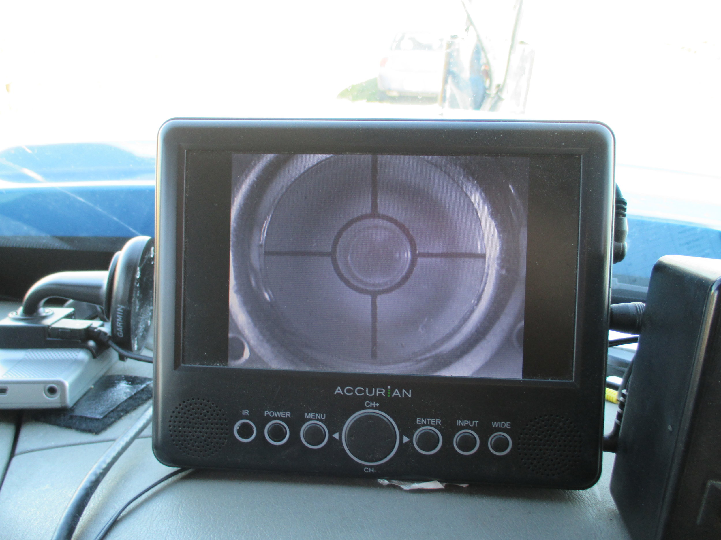
Fig 9.1: The leveling of the DOW at scanning location 1.

Fig 9.2: The leveling of the DOW at scanning location 2.
At both of our locations the DOW was facing east with the wind farm off to the left side of the DOW to the north. The wind farm was between 200 and 320 degrees.
The DOW deployment did not go to the original plan. We originally wanted to scan from several locations around the wind farm, however due to the time constraints we had to limit ourselves to one location. When we arrived at the first location, the wind farm was in the zero band so we had to change our spot. The DOW also did not work properly the first try. The first frequency was not working right and the data was very noisy as seen in Fig. 10. As we went through the experiment, the DOW slowly became not level. This wasn't an issue for our data however.
In order to correct our problems, we chose a location that would work and get good data. To fix the frequency issue, we just used the data from the second frequency which was working fine.

Fig 10: The radar date from frequency one was very noisy and wasn't able to be used.
While using the DOW, we used both RHI and PPI scans. For the PPI scans we used a number of elevation angles:
• .5, 1, 1.5, 2, 2.5, 3, 3.5, 4, 4.5, 5, 6, 7, 8, 9, 10, 12, and 15.
The azimuth rate for the PPI scans was 20 degrees per second.
For the RHI scans we used the following angles:
• 30, 180, 200, 210, 230, 240, 260, 270, 300
For the individual projects, we specifically looked at turbulence that was visible in the PPI and RHI scans. We were looking primarily at the velocity data to look at the effects of the wind turbines on the outgoing wind.
Some of the interesting things we saw while we were scanning included the interesting velocity
data. We also saw a dust devil that happened right next to the DOW that carried corn stalks high up
into the sky.
Ground Clutter Diagnosis
Using the radar data we can clearly see our dominant ground clutter objects. As seen in Fig. 11, ground clutter object are labeled. The trees SW of the DOW, or between 135 and 180 degrees in the radar data, create holes in the radar data.
Wind turbines also show up as ground clutter in the radar data and they are circled in Fig. 11. They show up very well in the reflectivity and velocity data.

Fig 11: Ground clutter labeled. The DOW velocity data (left) shows three areas of no returns. The picture on the right shows what is actually creating the ground clutter returns. Further to the left of the radar shows the other ground clutter returns, the wind turbines.
Data Description
During our deployment, the DOW created a total of 451 sweep files for a total file size of 2.0GB.
Data Analysis

WEB BONUS: Animated radar loop of the 3°, 3.5°, 4° and 4.5° velocity scans.
Analyzing the data there are plentiful interesting things to pick out of the radar images. For the purpose of our experiment we used both RHI and PPI scans. We are primarily looking at the velocity data for this experiment, however we included reflectivity scans as well.
Starting with the PPI scans, the wind farm was very visible on the on the reflectivity and the velocity scans. In Fig. 22, you can see the individual wind turbines that show up on the reflectivity scans. We filtered out much of the clutter from the reflectivity data and set the range to make the turbines pop out. Circled in Fig. 22 is much of the sets of wind turbines.
Starting with the velocity data, Figs. 12-15 are PPI scans starting with 4 degrees, increasing to 5, 6, then 9.
Starting with Fig. 12, the elevation angle is 4 degrees. Two areas of wind disturbance were generated downwind of the wind turbines that is easily seen. Circle 1 shows a very large area of lesser velocity values behind the field of wind turbines. Circle 2 shows a smaller area of disturbance behind another set of turbines.
In Fig. 13 the elevation angle is increased to 5 degrees. Circle 1 continues to show the large disturbance behind the wind farm higher up in the atmosphere. Circle 2 also shows the other area of disturbance behind another set of wind turbines.
In Fig. 14 the elevation angle is increased to 6 degrees. At this elevation three areas of wind disturbance become visible. The large area in circle 1 persists behind the large field of turbines. A new area in circle two is showing up behind a line of turbines. Finally continually showing up in circle 3 is the other area of disturbance. Also showing up more visibly at this elevation is turbulence being generated behind wind turbines. Inside circle 1 has areas of yellow velocities, or incoming velocities. This is wind being generated behind the wind turbines and blowing towards the radar opposite the mean wind. This is also easily identified in the RHI scan in Fig. 19.
Finally for the PPI scans in Fig. 15, the elevation angle was increased to 9 degrees. Still apparent in the velocity scan is the disturbance behind the large number of turbines in circle 1. Also in circle 2 there still is the disturbance behind the set of wind turbines.

Fig 12: Velocity scan at 4 degrees. The circled areas show the two dominant areas of wind disturbance. Circle 1 shows a large area of lesser wind velocity downwind from a large grouping of wind turbines. Circle 2 shows another area of disturbance that is more noticeable. Faster winds race around the wind turbines, while an area of lesser winds lies downwind from the set of turbines.

Fig 13: Velocity scan at 5 degrees. The circled areas show the two dominant areas of wind disturbance higher up. Circle 1 shows a large area of lesser wind velocity downwind from a large grouping of wind turbines. Circle 2 shows another area of disturbance that is still noticeable. Faster winds race around this wind turbines in circle 2, while an area of lesser winds lies downwind from the set of turbines.

Fig 14: Velocity scan at 6 degrees. The circled areas show three areas of wind disturbance. Circle 1 shows a large area of lesser wind velocity downwind from a large grouping of wind turbines. Inside circle one also shows some other effects of the wind turbines. At this elevation scan you can see incoming wind towards the radar directly behind the turbines sowing turbulence is forming. Circle 2 shows another area of disturbance that is also noticeable. Faster winds race around the wind turbines, while an area of lesser winds lies downwind from the set of turbines. Circle 3 shows a new area of wind disturbance that is showing up downwind from a set of wind turbines.

Fig 15: Velocity scan at 9 degrees. The circled areas show two areas of wind disturbance. Circle 1 shows a large area of lesser wind velocity downwind from a large grouping of wind turbines. Inside circle one also shows some other effects of the wind turbines. Also at this elevation scan you can see incoming wind towards the radar directly behind a few turbines showing turbulence. Circle 2 shows another area of disturbance that is also noticeable. Faster winds race around the wind turbines, while an area of lesser winds lies downwind from the set of turbines.
Moving onto the RHI scans, the velocity data was quite stunning and told a very clear story. Fig. 16 is at an angle of 30 degrees from the radar looking SE into the wind. This is near parallel to the wind vector, so the velocity data was very clear. Shown is the velocity data on the bottom is a very evident bulge in the wind over the town of Altona, Illinois.
There is a speed max in front of the town, and directly above and behind the town.
In Fig. 17 it is 230 degrees, or NW of the DOW looking downstream of the wind. This is on the edge of the wind farm and the wind turbines are visible in the reflectivity data (top). The velocity data shows a similar bulge of wind over the turbines with a speed max ahead of the turbines, and behind the turbines.
Fig. 18 is at 240 degrees from the radar still looking NW. Again the velocity data bulges over the wind turbines with a speed max ahead of and behind the turbines. The downstream effects of the wind turbines persist for quite some distance.
Fig. 19 is looking into the heart of the wind farm at 260 degrees, or NNW. Several wind turbines are visible in the reflectivity data (top). The velocity data (bottom) continually shows the bulging of the wind with speed maxes directly ahead of the turbines. However the speed max which is usually behind the turbines isn't as visible. It seems the wind turbines are very tightly packed and acting as one big block to the wind. The downstream effects persist for a very large distance from the final wind turbine. Also shown is turbulence being generated behind the turbines. The yellow velocity data is incoming winds behind the wind turbines. A very weak cyclonic turning to the wind is showing.
Fig. 20 is looking at 270 degrees from the radar, or straight north. Again in the reflectivity data (top) the wind turbines are visible. In the velocity data (bottom) the same bulge is apparent as with the other scans. The downstream effects of these turbines go on for a while. The first set of turbines created a bulge that subsides just before the second wind turbine. Then another bulge is formed. As with Fig. 19, turbulence is seen being generated behind the wind turbine with yellow incoming winds indicated by the arrow. This cyclonic flow is similar as Fig. 19.
Finally Fig. 21 is looking at 300 degrees towards the NE. This angle is looking into the zero band and the velocity data is a little skewed. However the turbines are still showing on the reflectivity data (top) and there is an effect showing in the velocity data (bottom). Much of the turbulence that is shown in this radar image is likely due to the changing wind direction with altitude. The surface winds were slightly towards the radar, while aloft they are angled away from the radar. While it may not be best for looking at the wind turbines, it does show a nice slice of the wind profile of the atmosphere.
Fig. 22 is a reflectivity image at 2 degrees. Circled are many of the wind turbines from the wind farm. This is just a small number of the nearly 100 wind turbines a part of the Bishop Hill wind farm.

Fig 16: An RHI scan at 30 degrees from the radar, looking SE. The velocity data (bottom) shows the strong incoming winds as this is nearly parallel to the wind vector. A bulge in the strong wind flow is also noticeable as the town of Altona, IL creates a block to the wind. Buildings can be seen as well in the missing velocity data.

Fig 17: An RHI scan at 230 degrees from the radar, looking NW. This is the first scan where wind turbines become visible in the reflectivity data (top). Using the velocity data (bottom) you can see the wind velocities change as wind bulges over the wind turbines. Speed maxes are right above each turbine and behind.

Fig 18: An RHI scan at 240 degrees from the radar, looking NW. Wind turbines are visible in this reflectivity data (top) like Fig 17. Wind is again seen bulging over the wind turbines (bottom) maxing just above the wind turbines. Also seen near the surface is incoming velocities showing that minor turbulence may be forming in the wake of the turbines.

Fig 19: An RHI scan at 260 degrees from the radar looking NNW. A large grouping of wind turbines is seen in the reflectivity data (top). Velocity data (bottom) is also excellent at this angle showing the large bulges over the turbines. Becoming visible better in the velocity data is the turbulence behind the turbines.

Fig 20: An RHI scan at 270 degrees from the radar looking N. Again the wind turbines are seen in the reflectivity data (top), and the velocity data (bottom) shows the same bulge in the velocities over the turbines. Seen behind the furthest turbine is an area of turbulence denoted by the yellow incoming winds.

Fig 21: An RHI scan at 300 degrees from the radar looking NE. In the reflectivity data (top) the wind turbines can be seen. The velocity data is a little skewed as it is looking in the zero band where the wind is near perpendicular to the radar beam. However velocity data still shows the winds bulging over the wind turbines and some turbulence shown behind the turbines.

Fig 22: Reflectivity data shows the individual wind turbines. Circled are the several groupings of wind turbines.